Why gradient descent works at all (and when it shouldn’t)

Gradient descent is a local procedure. It looks at the slope under its feet and moves downhill. Applied to a non-convex landscape with billions of parameters, it should get stuck constantly. It does not. Modern networks train reliably with what is essentially the simplest optimization algorithm we have, and the reasons are not yet fully understood. What we do know turns the question from "miracle" into "structured phenomenon," but the residual gap is real and worth taking seriously.

The puzzle in its classical form

The original framing was geometric. If GD finds good solutions, the loss landscape must be benign in some sense: maybe most local minima are also global, maybe saddle points are escapable in polynomial time, maybe the basin of attraction of bad minima is small. Theorems in this style exist for specific architectures (Choromanska et al. 2015 on the spin-glass connection; Kawaguchi 2016 on deep linear networks). The trouble is that they describe properties of a static loss surface and treat GD as a procedure that might or might not find the good parts. This decouples the optimizer from the landscape in a way that does not match what trained networks look like.

The newer framing reverses this. With sufficient overparameterization, the trajectory of GD through parameter space is itself the object of interest. Most directions of motion barely change the loss; the dynamics live on a low-dimensional submanifold; and which minimum GD reaches depends on initialization and step size in predictable ways. This is the implicit bias of GD: among the continuum of solutions that fit the training data, GD systematically picks specific ones.

A worked example

Consider the simplest overparameterized regression. One training point $x = [1, 1]^\top \in \mathbb{R}^2$ , target $y = 1$ , linear model $\hat{y} = w^\top x$ . The squared loss is

L(w) = \tfrac{1}{2}(w_1 + w_2 - 1)^2.

The set of minima is the line $w_1 + w_2 = 1$ , a 1-dimensional continuum. The Hessian is rank-1 with null space along $(1, -1)$ , so the loss surface is a flat-bottomed trough. Any point in the trough fits the data perfectly. The question is which point GD picks.

Geometrically, this is the generic situation in overparameterized models. With $d > n$ , the set of zero-loss solutions is a $(d - n)$ -dimensional affine subspace, and the Hessian is degenerate everywhere on it. There is no curvature to break the symmetry among solutions; any tiebreaker has to come from the optimizer.

Gradient descent with step size $\eta$ and initialization $w^{(0)} = 0$ updates as

w^{(t+1)} = w^{(t)} - \eta,(w_1^{(t)} + w_2^{(t)} - 1),[1, 1]^\top.

Every step moves $w$ along $(1, 1)$ , so the trajectory is confined to that direction. It converges to $w^* = (1/2, 1/2)$ , the unique minimizer along the gradient direction from the origin. This is the minimum $\ell_2$ -norm solution, and it is not an accident of this example: GD from zero in any overparameterized linear regression converges to the minimum-norm interpolator (Gunasekar et al. 2017 give the general result).

Loss landscape diagram showing the solution manifold and GD convergence point — **Figure 1.** The loss surface for a single overparameterized regression point. The solid line is the 1D continuum of minima; dashed lines are level sets of the loss. Gradient descent from the origin moves along $(1,1)$ and converges to the minimum-norm solution $w^* = (\tfrac{1}{2}, \tfrac{1}{2})$ , regardless of which point on the line is the true generative parameter 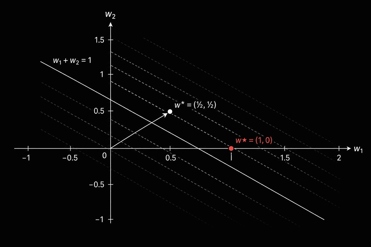$w^\star$ .

This is implicit bias in its cleanest form. The architecture does not constrain $w_1 = w_2$ . The loss does not prefer it. The optimizer chooses it.

When the bias is wrong

Implicit bias is only a feature when it points toward solutions that generalize. Suppose the true mechanism is $w^\star = (1, 0)$ : only the first feature matters. GD still returns $(1/2, 1/2)$ . On a test point $x = [1, 0]^\top$ where the truth is $y = 1$ , GD predicts $1/2$ . The model fits the training set perfectly and gets the test point half-right, not because capacity is missing, but because the optimizer's preferred minimum is the wrong one.

Diagram showing the generalization gap between GD's prediction and the true label on a test point — **Figure 2.** Implicit bias as generalization failure. Both $(1, 0)$ and $(\tfrac{1}{2}, \tfrac{1}{2})$ achieve zero training loss, but only the former predicts correctly on the test point $x = [1, 0]^\top$ . Capacity is sufficient; the optimizer's preferred minimum is the wrong one.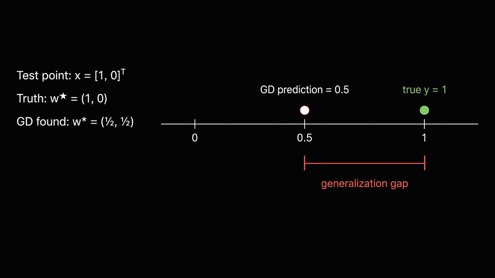

Scale this up and you get one version of why deep networks sometimes fail to learn features that are present in the data but not aligned with GD's geometric biases. Parity functions are the canonical case: they exist in the function class, but gradient signals near initialization are vanishingly small, and GD never finds them in reasonable time (Shalev-Shwartz et al. 2017; Abbe et al. 2022 sharpen this with the staircase property). Capacity is not the bottleneck. The dynamics are.

What the biological-plausibility debate actually says

A common framing has been that backpropagation is biologically implausible because it requires symmetric weight transport and non-local credit assignment. Recent results push back. Predictive coding networks compute backprop in a limit (Whittington and Bogacz 2017); equilibrium propagation produces gradients from energy minimization (Scellier and Bengio 2017). The substantive question is not whether the brain does backprop, but what minimal structural conditions let gradient-like signals emerge from local computation. That reframing makes the artificial-network puzzle more pointed, not less. Gradient signals are apparently a robust attractor for distributed learning systems.

The residual gaps

What we have is a partial story. Implicit bias is well characterized for linear models, deep linear networks, and matrix factorization. It is partially characterized for ReLU networks in the NTK regime, where training looks like kernel regression and the implicit bias inherits the kernel's geometry. It is poorly characterized in the feature-learning regime, which is where most useful neural network behavior actually lives.

Edge-of-stability dynamics (Cohen et al. 2021) make this concrete. In real training runs, the largest Hessian eigenvalue rises until it sits right at the stability threshold $2/\eta$ , and GD oscillates rather than monotonically decreasing. Classical convergence theory says this should not work. It works anyway, and we do not have a clean account of why this regime is stable, why it generalizes, or whether it is the same regime in which feature learning happens.

The honest summary is this. We have moved the question from "why does GD work at all" to "what is the implicit bias of GD in setting $X$ , and when does that bias align with good generalization." For some settings we have answers. For the settings that matter most, we have suggestive results and open problems. The miracle has been partially decomposed. The residue is not nothing.

This essay was written with AI assistance. All final arguments, edits, and responsibility are mine.